Tabular Data with Pandas

Pandas is the most popular Python tool for data analysis. It handles tabular data and has tons of nice features for manipulating text, grouping data by attributes, formatting dates, the list goes on… Even if you do not use tabular or csv data, you will likely end up using Pandas tools for some of their nice data-wrangling features. In general, if you have data that could be organized in an Excel spreadsheet or a table, you should use Pandas. This is particularly useful for data downloaded from places like NOAA and USGS where observations from individual meaurement stations are usually concatenated into a table of some kind. Pandas can be used to open data in CSV, HTML, JSON, XLS, Parquet, SQL, GBQ formats and more.

Earthquake Data Tutorial

For this tutorial we have grabbed the last 30 days of global earthquake activity from USGS (downloaded August 11th, 2025). The data only includes earthquakes of magnitude greater than or equal to 2.5.

import pandas as pd #import the pandas library

# open our csv file, this assumes it is in the top level of your VSCode workspace
df = pd.read_csv('global_30day_earthquakes.csv')

When we open a dataset, Pandas reads the data into an object called a ‘DataFrame’ which looks like a table.

# inspect our dataframe
df

	time	latitude	longitude	depth	mag	magType	nst	gap	dmin	rms	...	updated	place	type	horizontalError	depthError	magError	magNst	status	locationSource	magSource
0	2025-08-12T00:30:58.784Z	62.008000	-145.533400	9.800	2.60	ml	NaN	NaN	NaN	0.8700	...	2025-08-12T00:37:39.629Z	7 km SW of Copperville, Alaska	earthquake	NaN	0.300	NaN	NaN	automatic	ak	ak
1	2025-08-12T00:30:53.834Z	61.740900	-146.097200	42.400	2.60	ml	NaN	NaN	NaN	0.5700	...	2025-08-12T00:35:35.397Z	38 km S of Tolsona, Alaska	earthquake	NaN	3.200	NaN	NaN	automatic	ak	ak
2	2025-08-11T23:45:41.896Z	51.193700	160.859900	10.000	4.50	mb	25.0	135.00	2.2830	0.4400	...	2025-08-12T00:10:36.040Z	256 km SE of Vilyuchinsk, Russia	earthquake	7.30	1.883	0.069	61.0	reviewed	us	us
3	2025-08-11T21:24:31.503Z	41.242100	-116.714900	6.300	2.90	ml	14.0	144.57	0.3420	0.1627	...	2025-08-11T22:14:22.638Z	60 km NE of Valmy, Nevada	earthquake	NaN	3.300	0.260	12.0	reviewed	nn	nn
4	2025-08-11T21:02:42.456Z	51.651500	159.778700	35.000	5.00	mb	61.0	106.00	1.5390	0.6000	...	2025-08-12T00:35:51.040Z	170 km SSE of Vilyuchinsk, Russia	earthquake	6.76	1.859	0.043	175.0	reviewed	us	us
...	...	...	...	...	...	...	...	...	...	...	...	...	...	...	...	...	...	...	...	...	...
2658	2025-07-13T03:02:17.889Z	-22.593300	-68.014400	153.524	4.40	mb	29.0	89.00	0.3880	0.8700	...	2025-08-02T22:30:27.040Z	40 km NNE of San Pedro de Atacama, Chile	earthquake	7.46	5.557	0.138	15.0	reviewed	us	us
2659	2025-07-13T02:32:49.570Z	32.791833	-115.829333	4.810	2.62	ml	67.0	28.00	0.1032	0.2600	...	2025-08-02T22:22:55.040Z	17 km ENE of Ocotillo, CA	earthquake	0.20	0.640	0.121	131.0	reviewed	ci	ci
2660	2025-07-13T00:49:42.340Z	-9.885400	116.631100	54.034	4.10	mb	17.0	104.00	1.5440	0.4500	...	2025-07-25T02:12:15.040Z	128 km S of Taliwang, Indonesia	earthquake	8.08	5.198	0.174	9.0	reviewed	us	us
2661	2025-07-13T00:30:59.994Z	50.336900	-175.400000	10.000	2.80	ml	19.0	235.00	1.6530	0.7300	...	2025-07-22T21:41:02.040Z	191 km SSE of Adak, Alaska	earthquake	3.57	2.019	0.105	12.0	reviewed	us	us
2662	2025-07-13T00:11:12.440Z	-49.427300	-8.066900	10.000	4.50	mb	14.0	106.00	22.4470	0.6600	...	2025-07-25T01:58:47.040Z	southern Mid-Atlantic Ridge	earthquake	8.85	1.934	0.145	14.0	reviewed	us	us

2663 rows × 22 columns

# instead of looking at the whole table, lets see an overview of the information we have
df.info()

<class 'pandas.core.frame.DataFrame'>
RangeIndex: 2663 entries, 0 to 2662
Data columns (total 22 columns):
 #   Column           Non-Null Count  Dtype
---  ------           --------------  -----
 0   time             2663 non-null   object
 1   latitude         2663 non-null   float64
 2   longitude        2663 non-null   float64
 3   depth            2663 non-null   float64
 4   mag              2663 non-null   float64
 5   magType          2663 non-null   object
 6   nst              2498 non-null   float64
 7   gap              2496 non-null   float64
 8   dmin             2496 non-null   float64
 9   rms              2662 non-null   float64
 10  net              2663 non-null   object
 11  id               2663 non-null   object
 12  updated          2663 non-null   object
 13  place            2663 non-null   object
 14  type             2663 non-null   object
 15  horizontalError  2481 non-null   float64
 16  depthError       2662 non-null   float64
 17  magError         2470 non-null   float64
 18  magNst           2478 non-null   float64
 19  status           2663 non-null   object
 20  locationSource   2663 non-null   object
 21  magSource        2663 non-null   object
dtypes: float64(12), object(10)
memory usage: 457.8+ KB

We can see that the column ‘time’ has been recognized as a generic object, instead of a date. Let’s fix that by telling Pandas which column to interpret as a date type. The list above tells us that the date is the 0th column.

df = pd.read_csv('global_30day_earthquakes.csv', parse_dates=[0])

When we run df.info() again, we can see that time is now a datetime64 type. We can also see that the datetime units are nanoseconds, and that it is UTC time. One of the best features of Pandas is the ease with which it can handle and interpret dates.

df.info()

<class 'pandas.core.frame.DataFrame'>
RangeIndex: 2663 entries, 0 to 2662
Data columns (total 22 columns):
 #   Column           Non-Null Count  Dtype
---  ------           --------------  -----
 0   time             2663 non-null   datetime64[ns, UTC]
 1   latitude         2663 non-null   float64
 2   longitude        2663 non-null   float64
 3   depth            2663 non-null   float64
 4   mag              2663 non-null   float64
 5   magType          2663 non-null   object
 6   nst              2498 non-null   float64
 7   gap              2496 non-null   float64
 8   dmin             2496 non-null   float64
 9   rms              2662 non-null   float64
 10  net              2663 non-null   object
 11  id               2663 non-null   object
 12  updated          2663 non-null   object
 13  place            2663 non-null   object
 14  type             2663 non-null   object
 15  horizontalError  2481 non-null   float64
 16  depthError       2662 non-null   float64
 17  magError         2470 non-null   float64
 18  magNst           2478 non-null   float64
 19  status           2663 non-null   object
 20  locationSource   2663 non-null   object
 21  magSource        2663 non-null   object
dtypes: datetime64[ns, UTC](1), float64(12), object(9)
memory usage: 457.8+ KB

We can inspect the first few entries with df.head()

df.head()

	time	latitude	longitude	depth	mag	magType	nst	gap	dmin	rms	...	updated	place	type	horizontalError	depthError	magError	magNst	status	locationSource	magSource
0	2025-08-12 00:30:58.784000+00:00	62.0080	-145.5334	9.8	2.6	ml	NaN	NaN	NaN	0.8700	...	2025-08-12T00:37:39.629Z	7 km SW of Copperville, Alaska	earthquake	NaN	0.300	NaN	NaN	automatic	ak	ak
1	2025-08-12 00:30:53.834000+00:00	61.7409	-146.0972	42.4	2.6	ml	NaN	NaN	NaN	0.5700	...	2025-08-12T00:35:35.397Z	38 km S of Tolsona, Alaska	earthquake	NaN	3.200	NaN	NaN	automatic	ak	ak
2	2025-08-11 23:45:41.896000+00:00	51.1937	160.8599	10.0	4.5	mb	25.0	135.00	2.283	0.4400	...	2025-08-12T00:10:36.040Z	256 km SE of Vilyuchinsk, Russia	earthquake	7.30	1.883	0.069	61.0	reviewed	us	us
3	2025-08-11 21:24:31.503000+00:00	41.2421	-116.7149	6.3	2.9	ml	14.0	144.57	0.342	0.1627	...	2025-08-11T22:14:22.638Z	60 km NE of Valmy, Nevada	earthquake	NaN	3.300	0.260	12.0	reviewed	nn	nn
4	2025-08-11 21:02:42.456000+00:00	51.6515	159.7787	35.0	5.0	mb	61.0	106.00	1.539	0.6000	...	2025-08-12T00:35:51.040Z	170 km SSE of Vilyuchinsk, Russia	earthquake	6.76	1.859	0.043	175.0	reviewed	us	us

5 rows × 22 columns

We can see above that each entry gets a generic row index of 0, 1, 2,… That isn’t particularly useful for our analysis since the indices don’t mean anything physical. Let’s change that by telling Pandas which column to use as the index. In this case we will use the earthquake ID. These are unique alphanumeric strings assigned by USGS to each earthquake.

df = df.set_index('id')
df.head()

	time	latitude	longitude	depth	mag	magType	nst	gap	dmin	rms	...	updated	place	type	horizontalError	depthError	magError	magNst	status	locationSource	magSource
id
ak025aagkam9	2025-08-12 00:30:58.784000+00:00	62.0080	-145.5334	9.8	2.6	ml	NaN	NaN	NaN	0.8700	...	2025-08-12T00:37:39.629Z	7 km SW of Copperville, Alaska	earthquake	NaN	0.300	NaN	NaN	automatic	ak	ak
ak025aagka93	2025-08-12 00:30:53.834000+00:00	61.7409	-146.0972	42.4	2.6	ml	NaN	NaN	NaN	0.5700	...	2025-08-12T00:35:35.397Z	38 km S of Tolsona, Alaska	earthquake	NaN	3.200	NaN	NaN	automatic	ak	ak
us6000qzzz	2025-08-11 23:45:41.896000+00:00	51.1937	160.8599	10.0	4.5	mb	25.0	135.00	2.283	0.4400	...	2025-08-12T00:10:36.040Z	256 km SE of Vilyuchinsk, Russia	earthquake	7.30	1.883	0.069	61.0	reviewed	us	us
nn00902440	2025-08-11 21:24:31.503000+00:00	41.2421	-116.7149	6.3	2.9	ml	14.0	144.57	0.342	0.1627	...	2025-08-11T22:14:22.638Z	60 km NE of Valmy, Nevada	earthquake	NaN	3.300	0.260	12.0	reviewed	nn	nn
us6000qzz1	2025-08-11 21:02:42.456000+00:00	51.6515	159.7787	35.0	5.0	mb	61.0	106.00	1.539	0.6000	...	2025-08-12T00:35:51.040Z	170 km SSE of Vilyuchinsk, Russia	earthquake	6.76	1.859	0.043	175.0	reviewed	us	us

5 rows × 21 columns

We can investigate specific columns of the first 10 entries with the following syntax:

df[['place', 'mag','depth']].head(n=10)

	place	mag	depth
id
ak025aagkam9	7 km SW of Copperville, Alaska	2.6	9.800
ak025aagka93	38 km S of Tolsona, Alaska	2.6	42.400
us6000qzzz	256 km SE of Vilyuchinsk, Russia	4.5	10.000
nn00902440	60 km NE of Valmy, Nevada	2.9	6.300
us6000qzz1	170 km SSE of Vilyuchinsk, Russia	5.0	35.000
us6000qzyh	195 km SE of Vilyuchinsk, Russia	4.8	10.000
us6000qzvz	94 km NW of Copiapó, Chile	4.8	23.635
us6000qzv1	southeast of the Loyalty Islands	4.8	10.000
us6000qzux	115 km SE of Attu Station, Alaska	4.2	35.000
nn00902450	55 km NE of Valmy, Nevada	2.5	11.300

We can grab summary statistics of our entire DataFrame using df.describe().

df.describe()

	latitude	longitude	depth	mag	nst	gap	dmin	rms	horizontalError	depthError	magError	magNst
count	2663.000000	2663.000000	2663.000000	2663.000000	2498.000000	2496.000000	2496.000000	2662.000000	2481.000000	2662.000000	2470.000000	2478.000000
mean	35.686975	24.620066	44.237501	4.140421	51.969976	138.648778	1.958450	0.735855	7.573879	4.463947	0.093915	86.439871
std	28.067148	142.590874	83.846288	0.893920	39.714453	59.363062	2.873961	0.294644	3.474638	17.009364	0.050587	141.302986
min	-63.245700	-179.983200	-2.360000	2.500000	0.000000	12.000000	0.000000	0.050000	0.080000	0.000000	0.001186	2.000000
25%	19.406700	-149.969300	10.000000	3.300000	24.000000	101.000000	0.527750	0.560000	5.440000	1.869000	0.056000	15.000000
50%	51.341200	120.729800	17.413000	4.400000	40.000000	131.000000	1.351000	0.730000	7.970000	1.961000	0.088000	30.000000
75%	52.897450	159.673300	35.000000	4.700000	68.000000	184.000000	2.246000	0.930000	9.850000	6.337750	0.121000	88.000000
max	83.270300	179.909500	638.859000	8.800000	338.000000	352.000000	33.879000	2.340000	22.620000	850.600000	0.371000	1144.000000

Looks like the largeset earthquake in the last 30 days was an 8.8 (see column mag, row max), and the average earthquake size was 4.1 with a standard deviation of 0.89. We can use features like nlargest to quickly sort through our data. If we use nlargest on mag we can find the n largest earthquakes. Let’s do 20.

df.mag.nlargest(n=20)

id
us6000qw60    8.8
us7000qdyl    7.4
us7000qd1y    7.3
us6000qvsf    7.0
us6000qw6q    6.9
us6000qxt4    6.8
us7000qcik    6.7
us6000qw1a    6.6
us6000quy1    6.6
us7000qdz2    6.6
us7000qdyw    6.6
us7000qdye    6.6
us6000qvpp    6.5
us6000qxsv    6.4
us6000qwiq    6.4
us6000qugg    6.3
us6000qxzw    6.2
us6000qwuh    6.2
us6000qw6s    6.2
us6000qvbw    6.2
Name: mag, dtype: float64

Now let’s look at some of the more interesting details, like where are these earthquakes happening? We can see there is a column called place.

df['place'].head()

id
ak025aagkam9       7 km SW of Copperville, Alaska
ak025aagka93           38 km S of Tolsona, Alaska
us6000qzzz       256 km SE of Vilyuchinsk, Russia
nn00902440              60 km NE of Valmy, Nevada
us6000qzz1      170 km SSE of Vilyuchinsk, Russia
Name: place, dtype: object

It looks like the place descriptor has lots of extra text. We want something more concise so that we can categorize the earthquakes by larger areas (e.g., Alaska). Let’s create a new column, called loc where we take just the last phrase in the place descriptor.

The next step is a little nuanced, because you have to use a regex (regular expression) pattern to find what we are looking for. Regex is a powerful tool for parsing text and matching strings of various formats. We won’t teach it here, because ChatGPT is very good at generating regex patterns to find exactly what you need. The pattern used here will isolate the text after the comma in the place descriptor. If there isn’t a comma, then we will take the whole string.

# We'll try to get the last comma-separated part of the `place`, or the whole string if there is no comma
df['loc'] = df['place'].str.extract(r'(?:,\s*)([^,]+)$')

# If there are entires without a comma (like "Fiji region"), fill them with the original value
df['loc'] = df['loc'].fillna(df['place'])

# compare what we had in 'place' with what we have in 'loc'
print(df[['place', 'loc']].head())

                                          place     loc
id
ak025aagkam9     7 km SW of Copperville, Alaska  Alaska
ak025aagka93         38 km S of Tolsona, Alaska  Alaska
us6000qzzz     256 km SE of Vilyuchinsk, Russia  Russia
nn00902440            60 km NE of Valmy, Nevada  Nevada
us6000qzz1    170 km SSE of Vilyuchinsk, Russia  Russia

There could be many earthquakes in the same country, and none in another. Let’s look at a list of the unique values in the loc column.

df['loc'].unique()

array(['Alaska', 'Russia', 'Nevada', 'Chile',
       'southeast of the Loyalty Islands', 'Mexico', 'Turkey',
       'New Zealand', 'Vanuatu', 'Peru', 'CA', 'Tonga',
       'south of the Kermadec Islands', 'Philippines', 'Indonesia',
       'Timor Leste', 'Colombia', 'Sea of Okhotsk', 'Guam', 'Guatemala',
       'Washington', 'south of the Fiji Islands', 'Wyoming',
       'Dominican Republic', 'Taiwan', 'Canada', 'Puerto Rico',
       'western Indian-Antarctic Ridge', 'central Mid-Atlantic Ridge',
       'Burma (Myanmar)', 'Arizona', 'Macquarie Island region',
       'Azerbaijan', 'Indiana', 'Ethiopia', 'Chagos Archipelago region',
       'Argentina', 'Japan', 'Papua New Guinea', 'Tanzania',
       'Japan region', 'Uzbekistan', 'Oregon', 'Hawaii', 'Afghanistan',
       'Fiji', 'Tajikistan', 'California', 'U.S. Virgin Islands', 'Texas',
       'Greece', 'Solomon Islands', 'Reykjanes Ridge', 'West Chile Rise',
       'southern Mid-Atlantic Ridge', 'New Mexico', 'Banda Sea',
       'New Jersey', 'Kansas', 'Kyrgyzstan', 'Saint Eustatius and Saba ',
       'east of the Kuril Islands', 'Iran', 'Bouvet Island region', 'MX',
       'Haiti', 'Fiji region', 'Nicaragua', 'El Salvador', 'Brazil',
       'Pacific-Antarctic Ridge', 'China', 'Pakistan', 'Portugal',
       'Venezuela', 'Costa Rica', 'Arkansas', 'Gulf of Alaska',
       'northern Mid-Atlantic Ridge', 'South Sandwich Islands region',
       'Montana', 'Saudi Arabia', 'Russia Earthquake', 'India',
       'Mariana Islands region', 'Mauritius - Reunion region', 'Idaho',
       'Burundi', 'Ecuador', 'Djibouti', 'Iceland', 'India region',
       'Northern Mariana Islands', 'east of the South Sandwich Islands',
       'Kermadec Islands region', 'Bolivia', 'west of Macquarie Island',
       'Antigua and Barbuda', 'New Caledonia',
       'Azores-Cape St. Vincent Ridge', 'Wallis and Futuna', 'Oklahoma',
       'Scotia Sea', 'Kazakhstan', 'Yemen', 'Madagascar',
       'Easter Island region', 'Falkland Islands region',
       'Balleny Islands region', 'southeast of Easter Island',
       'North Pacific Ocean', 'north of Ascension Island',
       'Iceland region', 'Anguilla', 'Malaysia', 'New Zealand region',
       'northern East Pacific Rise', 'off the coast of Oregon',
       'Owen Fracture Zone region', 'Carlsberg Ridge',
       'east of the North Island of New Zealand', 'south of Tonga',
       'Alaska Earthquake', 'Kuril Islands',
       'near the north coast of Greenland', 'Mauritius', 'Panama',
       'central East Pacific Rise', 'Spain'], dtype=object)

Maybe we are only interested in larger earthquakes that are more likely to be felt. We can create a new DataFrame that only contains earthquakes larger than 4.0.

df_mag4 = df[df['mag'] >= 4.0]

Now we can start plotting. Pandas and matplotlib work well together to naturally generate plots that have nicely labeled axes. You will have to define the details of the plots, but Pandas makes it very easy to subset/select data by different columns, date ranges, etc.

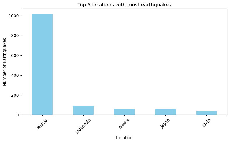
Plot Top 5 Most Earthquakes by Location

import matplotlib.pyplot as plt

# count how many earthquakes per country
counts = df_mag4['loc'].value_counts()

# take the top 5
top5 = counts.head(n=5)

fig, ax = plt.subplots(figsize=(8,5))
top5.plot(kind='bar',color='skyblue')
ax.set_title('Top 5 locations with most earthquakes')
ax.set_xlabel('Location')
ax.set_ylabel('Number of Earthquakes')
ax.tick_params(axis="x", rotation=45)

plt.tight_layout()

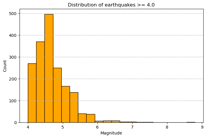
Plot a Histogram of Earthquake Magnitudes

fig, ax = plt.subplots(figsize=(8,5))
ax.hist(df_mag4['mag'],bins=20,color='orange',edgecolor='black')
ax.set_title('Distribution of earthquakes >= 4.0')
ax.set_xlabel('Magnitude')
ax.set_ylabel('Count')
ax.grid(axis='y',linestyle='--')

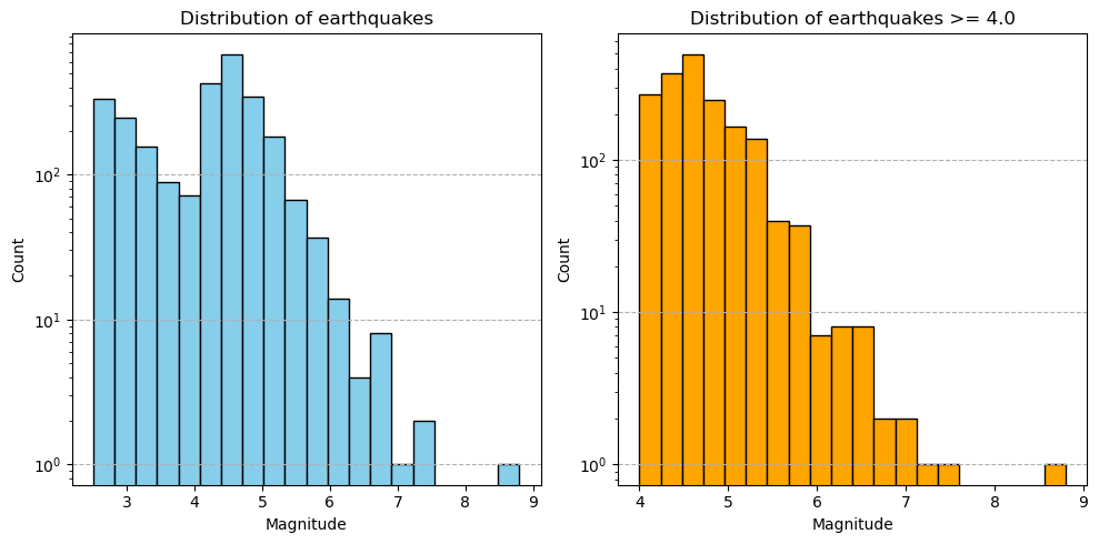
Plot a Histogram From Both Datasets with Log Axis

fig, ax = plt.subplots(1,2,figsize=(10,5))

ax[0].hist(df['mag'],bins=20,color='skyblue',edgecolor='black')
ax[0].set_title('Distribution of earthquakes')
ax[0].set_xlabel('Magnitude')
ax[0].set_ylabel('Count')
ax[0].grid(axis='y',linestyle='--')
ax[0].set_yscale('log')

ax[1].hist(df_mag4['mag'],bins=20,color='orange',edgecolor='black')
ax[1].set_title('Distribution of earthquakes >= 4.0')
ax[1].set_xlabel('Magnitude')
ax[1].set_ylabel('Count')
ax[1].grid(axis='y',linestyle='--')
ax[1].set_yscale('log')

plt.tight_layout()

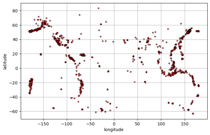
Scatter Plot of Earthquake Locations

fig, ax = plt.subplots(figsize=(8,5))

ax.scatter(df['longitude'],df['latitude'],s=10, alpha=0.6,c='red',edgecolors='black')
ax.set_xlabel('longitude')
ax.set_ylabel('latitude')
ax.grid(True)

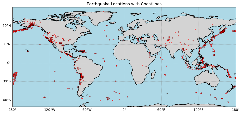
Add a Map to Scatter with Cartopy

import cartopy.crs as ccrs
import cartopy.feature as cfeature

# Create a GeoAxes with PlateCarree projection (standard lat/lon)
fig = plt.figure(figsize=(12,10))
ax = plt.axes(projection=ccrs.PlateCarree())

# Add coastlines and land features
ax.coastlines(resolution='110m')
ax.add_feature(cfeature.LAND, facecolor='lightgray')
ax.add_feature(cfeature.OCEAN, facecolor='lightblue')

# Scatter earthquake points
ax.scatter(df['longitude'], df['latitude'], s=10, c='red', alpha=0.6,
           edgecolors='k', linewidth=0.3, transform=ccrs.PlateCarree())

# Add gridlines with labels
gl = ax.gridlines(draw_labels=True, linewidth=0.5, color='gray', alpha=0.5, linestyle='--')
gl.top_labels = False
gl.right_labels = False

ax.set_title('Earthquake Locations with Coastlines')

plt.show()

Exercises

1. Update the scatter plot, such that the color of each dot reflects the magnitude of the earthquake.

2. Same idea as option (1), but make the size of each dot reflect the magnitude of the earthquake.

3. Create a new table that only contains earthquakes from Russia. Investigate the distribution of earthquake magnitudes in Russia in the last 30 days. Plot just the relevant region, and include some coloring or sizing of the scatter to highlight the biggest earthquakes.

Content for this tutorial was inspired by following an assignment from the Earth and Environmental Science Databook. The assignment can be found here.